Serving Playbook by Model Architecture

The goal is to acquire the ability to independently derive serving designs by only looking at a new model's config.json and model card.

Architecture Classification: You should be able to identify whether a model is GQA, MLA, DSA, or hybrid based on a few fields.
KV Cache Sizing: Depending on the architecture, you should decide whether to calculate it manually or measure it, and from that value, you can inversely calculate the number of concurrent users.
Choose Parallelization: You should be able to decide whether to use TP, EP, or DP attention based on the architecture and traffic volume.
Hardware Compatibility Verification: You should be able to determine if this model runs on your GPU and if it's the optimal path for it to run.
Root Cause Analysis from Symptoms: Track and resolve issues like the model not using tools or memory filling up quickly.

Prerequisites #

Transformer basic structure (layers, attention, FFN)
Why KV cache exists
Difference between prefill and decode
Parallelization: TP, PP, EP, DP
Basic concepts of quantization

What You Will Learn #

Differences between MHA, MQA, GQA, and why GQA became the standard
What MLA compresses
How sparse attention and indexers work
How linear attention's state differs from KV cache
MoE routing and expert parallelism
Why compute capability (sm_XX) restricts deployment

Architecture Determination #

When serving models at scale, you need to solve problems in situations like these:

Insufficient Context: Started with 128k, but customers began inputting entire contracts -> need to switch to a 1M-supported model, which is usually a different architecture.
Cost Mismatch: Traffic increased tenfold, leading to a GPU expansion quote... which is prohibitively expensive -> switching to an MoE with fewer active parameters can handle it without expansion.
Insufficient Quality: The coding agent's failure rate doesn't meet the target.

If it's due to context, KV cache is the top priority; if it's due to cost, expert parallelization is the top priority. You need to be able to make such judgments. Approaching it simply by "switching to a better model" prevents you from determining what to check and optimize.

First, let's consider scenarios where model serving is necessary and think through them.

When Starting a New Service and Serving a New Model #

Let's start with a situation where you have GPUs and a fixed budget, and you need to decide which model to deploy.

A common mistake is to pore over benchmark leaderboards, pick the model with the highest SWE-bench score, and then despair when you realize it won't run on your GPU.

Let's start by looking at the available hardware and pruning candidates.

SM #

Below, you'll see notations like sm_89, which refer to GPU generations.

It's called CUDA compute capability, and this number determines which hardware a kernel runs on.

sm_86    Ampere consumer (RTX 3090)
sm_89    Ada (RTX 4090)
sm_90    Hopper (H100, H200)
sm_100   Blackwell datacenter (B200, B300)
sm_120   Blackwell workstation (RTX 5090, RTX PRO)

A larger number doesn't necessarily mean it includes all previous generations; sometimes, a kernel written for sm_100 won't run on sm_120.

RTX 4090 two cards (sm_89)
  DSA architectures are out — sparse attention kernels only exist for sm_90 or higher
  Large MoE is out — won't fit in 48GB
  → GQA dense 20~30B class, or small hybrid

H200 eight cards (sm_90, 1,128GB)
  Most architectures are possible
  → Need to narrow down by workload

B300 rack (sm_100)
  Architectures with NVFP4 checkpoints are advantageous
  Models without them fall back to FP8, losing memory benefits

NVFP4 is a 4-bit floating-point format that stores weights and KV cache at 4 bits per element. Since only 16 values can be represented with 4 bits, it cannot be used as-is. Therefore, 16 values are grouped into a block, and each block has its own scale value. The actual value is the 4-bit value multiplied by that scale. Since neural network weights tend to have locally similar magnitudes, matching the scale at the block level allows even 16 steps to approximate the block's distribution well.

Compared to FP8, it's like this:

             Memory        Tensor Core Throughput      Hardware Support
FP8          1/2 (vs BF16)   2x                        Hopper or higher
NVFP4        1/4             4x                        Blackwell datacenter only

If memory is halved, twice the KV cache fits on the same GPU, increasing concurrency. If throughput doubles, prefill becomes twice as fast. This is usually why B300s are purchased.

The problem is that not just any model can run with NVFP4. A checkpoint quantized to NVFP4 must be distributed separately for the model; otherwise, you have to create it yourself, which requires calibration data and validation. Models without such checkpoints fall back to FP8, meaning you'd be using sm_100 hardware but only getting the performance achievable on sm_90.

Therefore, if you have a B300 rack, first check if the candidate model has publicly available NVFP4 checkpoints. Names often appear like nvidia/GLM-5.2-NFFP4.

Now that we've pruned candidates based on hardware, we need to understand the nature of the requests to be processed next, i.e., the workload, and branch accordingly.

Frequently handles 200k token documents
-> DSA or Hybrid; GQA's KV cache can't handle it

Short conversations and many concurrent users
-> GQA dense is sufficient; no need for complex architectures

Images are involved
-> Early fusion architectures only; others cannot handle it at all

Once you reach this point, the candidates will be narrowed down to three or four, and then you can compare their benchmark scores.

Operating with Handed-Over Configurations #

When a model and hardware are already set up and serving, and you're tasked with improving it, it's common in practice to operate without knowing why it's configured this way, with nothing to decide yourself.

python3 -m sglang.launch_server \
  --model nvidia/GLM-5.2-NVFP4 \
  --tensor-parallel-size 8 \
  --quantization modelopt_fp4 \
  --tool-call-parser glm47 \
  --reasoning-parser glm45 \
  --chunked-prefill-size 16384 \
  --mem-fraction-static 0.80

Here's a checklist of things to check:

Why is --kv-cache-dtype missing?
Why isn't --attention-backend specified?
What are these parser names glm47 glm45?
Why is --mem-fraction-static set to 0.80?

Not knowing these can lead to two types of accidents: one where you delete something necessary and a feature silently dies, and another where you add a flag and override the engine's automatic optimization.

If you get these wrong, the model might fail to launch, or it might launch but run slowly. For an MoE model, if you don't enable expert parallelism, it will still run, but expert weights will be replicated across all GPUs, reducing KV cache space and cutting concurrent users by more than half, leading to silent losses. Or, for a DSA model, specifying FP8 for kv_cache_dtype might override the engine's decision for optimal precision, resulting in acceptable performance without errors, but it's simply not ideal.

Now, let's look at each one. There are many things to consider, such as KV cache shape, parallelization strategy, kernel requirements, caching layer compatibility, and software version gating.

Serving by Attention Architecture - GQA #

Representative GQA models include Qwen3.6-27B, Qwen3 dense series, and Llama series.

GQA (Grouped-Query Attention) is a method where multiple attention heads share a single set of K and V.

It reduces the KV cache by 1/4 to 1/8 by sharing what was previously stored separately for each head, now at the group level.

MHA   [Head1:K,V][Head2:K,V][Head3:K,V][Head4:K,V]    4 sets of K,V
GQA   [Head1,2 : K,V      ][Head3,4 : K,V      ]    2 sets of K,V
MQA   [Head1,2,3,4 : K,V                       ]    1 set of K,V

As of 2026, this is the most widely used method, and all three architectures discussed later address the limitations left by this method in different ways.

First, let's understand why GQA was needed.

Why KV Cache Grows #

Attention is performed in parallel across multiple heads. Each head views the sentence from a different perspective.

Roles diverge, such as a head for grammar or a head for tracking referents.

Each head creates three vectors: Q (query), K (key), and V (value). It then calculates a score using the dot product of Q and K, and retrieves the V corresponding to the higher score.

During the generation phase, previously computed K and V are stored. To prevent recalculating 499 tokens when generating the 500th, they are pre-cached and stored. This is the KV cache.

The original method, MHA, has separate K and V for each head.

KV cache = 2 × number of layers × number of heads × head dimension × sequence length × bytes
          ↑                ↑
          K and V          Separate for each head

If there are 32 heads, 32 sets are stored; if there are 48 layers, this repeats 48 times. Let's plug in some numbers:

27B class model, MHA 32 heads, head dimension 128, 48 layers, FP8

KV per token = 2 × 48 × 32 × 128 × 1 = 393,216 bytes ≈ 384 KB
One 32K context user = 384 KB × 32,768 ≈ 12.6 GB

From one H200 (141GB), subtracting 27GB for weights leaves 114GB
→ 9 concurrent users

This means the service can only handle about 9 concurrent users.

Where MQA Failed #

The simplest solution is to have only one set of KV, maintaining 32 query heads but sharing all referenced KVs. This is MQA, Multi-Query Attention.

The KV cache becomes 1/32. In the calculation above, it shrinks from 12.6GB to 0.39GB, and concurrent users increase to 290.

However, while the memory issue was solved, the problem was a drop in quality. The structure was designed for each head to view from a different perspective, but unifying the information to be referenced reduced the diversity of perspectives.

Grouping #

GQA, therefore, avoids extreme sharing. It groups query heads, and each group has one set of KV. If there are 32 queries and 8 KVs, 4 queries share one KV, and the cache becomes 1/4.

The reason for minimal quality loss is that query heads within a group tend to look at similar things anyway. Instead of forcibly grouping heads with entirely different perspectives, dividing them into appropriate sizes allows each group to maintain its own perspective.

MQA broke this property by merging 32 heads into one, while GQA preserved it by grouping them in fours.

Method     KV Cache    Quality       Adoption
─────────────────────────────────────
MHA        Baseline    Highest       Early models
MQA        1/32        Degraded      Some models
GQA        1/4~1/8     Nearly Maintained  Current standard

Since all layers have the same structure, if we calculate KV:

Qwen3.6-27B (48 layers, 8 KV heads, head dimension 128, FP8)

KV per token = 2 × 48 × 8 × 128 × 1 = 98,304 bytes ≈ 96 KB
One 32K context user ≈ 3.1 GB
114 GB available → 36 concurrent users

If parallelizing, only TP will be used. Since there are no experts, EP is not an option, and as it's standard attention, there's no benefit to DP attention.

There are four ways to divide, but GQA dense eliminates three.

EP    A method for dividing experts, but dense models have no experts.
DP    The reason to separate attention is to prevent replication of compressed KV,
      but GQA does not compress, so there's no reason to separate it.
PP    Divides layers by depth. Communication is less, but GPUs work sequentially,
      so the speed of a single request doesn't improve. Rarely used in inference.

TP size can be set based on latency requirements. In practice, four TP2 instances showed 34% higher throughput than one TP8 instance, but the inter-token latency was about 42% worse.

One TP8 instance    Eight cards form one team. Eight cards process one request.
Four TP2 instances      Four teams of two cards each. Each team processes a different request.

In practice, four TP2 instances have 34% higher throughput and 29% shorter time to first token.

If latency requirements are strict, use a larger TP; if there's leeway, reduce TP and increase replication.

Kernels and caching can be left to automatic selection based on hardware generation via the standard path, and prefix caching also works as-is. This is because if the block hash is the same, the KV is bit-for-bit identical.

You can also attempt to reduce KV cache size through quantization.

TP2, FP8 standard
  KV per token = 2 × 48 × 8 × 128 × 1 = 96 KB
  One user ≈ 3.1 GB
  From two cards with 282 GB, subtracting 27 GB for weights leaves 255 GB
  → 82 concurrent users

If multiple requests start with the same system prompt, that part of the KV is identical each time. If you compute it once and reuse it, you can skip prefill, which is prefix caching.

In GQA, this just works because if the block hash is the same, the KV is bit-for-bit identical. Subsequent architectures have conditions here.

There's no need to worry about kernels either; since it's standard attention, the engine automatically selects them to match the hardware generation.

python -m sglang.launch_server \
  --model-path Qwen/Qwen3.6-27B \
  --tp-size 2 \
  --quantization fp8 --kv-cache-dtype fp8_e5m2 \
  --chunked-prefill-size 4096 \
  --enable-metrics

GQA Limitations #

In dense architectures, as parameters grow, the computation per token increases proportionally. At scale, this isn't cost-competitive, and by 2026, all large open-weight models have shifted to MoE.

Even if the KV cache is reduced by a factor of four, its growth property remains proportional to length, so at 1M context, it becomes unmanageable again. Even 1/4 is considered large.

These two limitations led to the following considerations and techniques:

Need to reduce KV cache further -> MLA
Need to reduce the reading scope -> DSA
Let's eliminate length dependency -> Hybrid

MLA, Compressing the KV Cache #

Representative models include DeepSeek V2/V3/V3.2 and the Kimi K2 series.

MLA (Multi-head Latent Attention) is a method that compresses K and V into low-dimensional vectors for storage and then expands them back from those vectors when calculating attention.

GQA   Several heads share one set of K,V      → Reduces the number of sets
MLA   Compresses K,V entirely into smaller vectors        → Reduces the size of a single set

If GQA is a sharing solution, MLA is about making the storage itself smaller.

High compression rates, yielding 7-14x savings, have been reported. However, it has poor compatibility with parallelization, creating new deployment challenges.

GQA reduced the cache by a factor of four, but to reduce it further, KV heads would need to be reduced, which would degrade quality.

32 queries, 8 KV   4 share. Quality maintained.
32 queries, 4 KV   8 share. Quality begins to waver.
32 queries, 1 KV   Same as MQA. Quality degradation confirmed.

GQA can only adjust how many share; if you push it too far, problems like MQA arise.

DeepSeek's goal was API cost competitiveness. Since KV cache determines the number of concurrent users, and the number of concurrent users determines revenue per GPU, reducing the cache directly translates to cost savings, so they began aggressively cutting it down.

Dimensionality Reduction #

Therefore, the attempt was made to reduce the size of the KV cache itself, rather than just the number of shared instances.

If you line up the K and V of 32 heads, you'll find many similar components. Even if each head views from a different perspective, they don't see entirely different things. Removing this redundancy allows them to be stored in much lower dimensions, reducing storage even while keeping the number of heads the same.

When storing   K, V  →  [Compression Matrix]  →  Latent Vector (low-dimension)
When using   Latent Vector  →  [Restoration Matrix]  →  K, V for each head

It's like keeping meeting documents as summaries instead of originals and restoring them when needed. Since the restoration matrix is determined through learning, the model itself learns what to discard and what to retain.

RoPE, which contains positional information, has poor compatibility with compression, so a separate path is maintained for it. For initial learning, it's sufficient to compress but handle positional information separately.

Challenges of MLA Serving (Redundant Storage) #

Here lies the challenge of MLA serving.

If attention is divided by TP, heads must be distributed among GPUs, but latent projection in MLA doesn't cleanly separate by head.

Ultimately, multiple GPUs end up storing the same latent vector redundantly. If TP=8, the cache is replicated 8 times, effectively losing the memory saved by compression due to replication.

Thus, a method emerged to run only the attention layers with DP. Each GPU only needs to hold the KV for the requests it's responsible for.

Attention Layer (DP=8)
  GPU 0~3 : Fully process request group A   ← Holds only its own KV
  GPU 4~7 : Request group B
            No communication between groups

MoE Layer (EP=32)
  The same 32 cards now handle experts in a divided manner

According to measurements by the AMD ROCm team, in the 64-128 concurrent request range, TP+EP showed 52% higher throughput than DP+EP, even with KV replication.

The reason lies in the nature of DP: each GPU receives requests independently, so if there are few requests, some groups remain idle. TP, however, processes a single request across multiple GPUs, so all GPUs work even with small batches.

If memory is sufficient and latency is a priority, use TP; if batch size needs to be increased, use DP.

DeepSeek V3 Serving #

Since it handles KV stored in a compressed form, standard attention kernels do not apply directly.

--attention-backend flashinfer     # SGLang, FlashInfer's MLA path
--enable-flashinfer-mla            # Kimi K2 series may require explicit specification

vLLM reads the attention structure from config.json and automatically routes to the MLA path. No separate flag is needed.

# vLLM, DeepSeek V3, 8×H200
vllm serve deepseek-ai/DeepSeek-V3 \
  --tensor-parallel-size 8 \
  --dtype fp8 --kv-cache-dtype fp8 \
  --max-model-len 131072 \
  --gpu-memory-utilization 0.92

# For large scale, EP + DP attention
vllm serve deepseek-ai/DeepSeek-V3 \
  -dp 8 --enable-expert-parallel \
  --dtype fp8 --kv-cache-dtype fp8

For Blackwell (B200), quantization with --kv-cache-dtype nvfp4 can achieve an additional 50% saving compared to FP8, while on Hopper, FP8 is the upper limit without hardware support.

Remaining Issues #

Since parallelization choices reverse based on concurrency, they must be re-evaluated if traffic patterns change.

A greater limitation is that even with a 7-14x reduction, it still grows proportionally with context length. For 1M context, it's still insufficient.

DSA, Selecting Tokens to Attend To #

Representative models include DeepSeek V3.2, GLM-5.1/5.2, and DeepSeekV4.

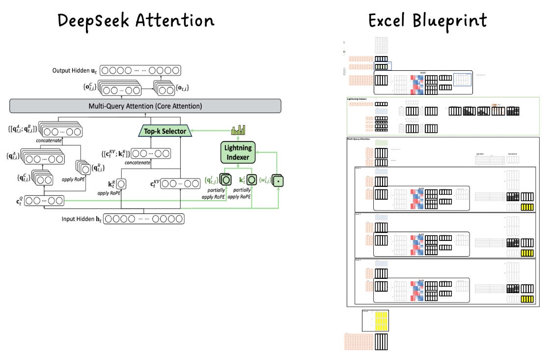
DSA (DeepSeek Sparse Attention) is a method that reduces reading, not storage.

Before calculating attention, it uses a lightweight filter to select k relevant tokens and only computes attention precisely on those.

Standard Attention: Compares with all 1 million tokens, computation is quadratic to length.
DSA: Selects only 2,048 tokens with a filter, then compares, computation fixed to k.

Whether the context is 100k or 1M, the actual tokens attended to are a fixed k, so attention cost remains almost constant even as length increases. This is why 1M context models use this method.

MLA significantly reduced storage, but two problems remained:

Memory still scales with length, and even compressed, 1 million items is large.

Also, computation increases quadratically; if there are N tokens, there are N^2 Q-K pairs. Even if storage is reduced, this computation remains the same.

Context Length     Attention Computation
─────────────────────────────
    1,000        1 million times
   10,000        100 million times
1,000,000        1 trillion times

Which Tokens to Discard? #

There's a technique called sliding window that only looks at N tokens. While it makes computation linear, it has the characteristic of missing important information far away. Tasks that require referencing clauses from the beginning of a 1 million token document would fail with this.

There are also fixed patterns like sampling at regular intervals or dividing into blocks. These reduce computation, but which tokens are important depends on the content, and fixed patterns cannot reflect that.

The third is selecting based on content, which is accurate, but if the judgment itself becomes expensive, it loses its meaning. There's no point in saving attention if you spend just as much on filter computation.

Extremely Lightweight Filters #

DSA uses the third method of selecting based on content, but makes the filter very cheap. This is the Lightning Indexer.

[KV of 1 million tokens]
       ↓
[Lightning Indexer]      Calculates relevance scores only via low-dimensional projection
       ↓
[Select top 2,048]    Based on GLM-5.2
       ↓
[Precise Attention]         Only this part is expensive

It's like writing a thesis in a library: instead of reading all 1 million books, you ask the librarian to pull out 2,000 relevant books and only read those thoroughly.

Unlike precise attention, the indexer only needs to assign approximate ranks, making it much cheaper. Indexer keys are computed once for each KV item, stored in GPU memory, and not recreated every time.

Since the top k is fixed, attention cost barely increases with longer contexts. As a side effect, irrelevant information is filtered out, making it robust to noise.

This is what DSA has solved. It has become independent of quadratically increasing attention, and for contexts up to about 128K, this is sufficient.

Indeed, DeepSeek V3.2 was released with this configuration.

However, the total cost of the model is not entirely independent of length. A new indexing step has been introduced before attention, and its cost has not yet been fully accounted for. At 128K, this cost is negligible compared to attention savings, but at 1M, it becomes a problem.

When the Indexer Becomes a Bottleneck and IndexShare #

For the indexer to select the top 2,048, it must scan all candidates. Since it's choosing from 1 million items, it will score all 1 million.

Attention    Calculates only with top 2,048      Fixed, regardless of length
Indexer    Scores all 1 million items   Increases proportionally with length

Attention is fixed, but the indexer still scales with length. At 128K, this value is small enough to be negligible compared to attention savings, but at 1M, it becomes 8 times larger.

Here, the number of layers is multiplied. While a single score calculation is a low-dimensional projection and much cheaper than attention calculation, with 61 layers, it means 61 million operations for every token generated. Even if the cost per item is small, this can become larger than attention.

You can't eliminate the indexer because you need to know what to select to skip attention... The only remaining path is to reduce the number of calls.

The characteristic that adjacent layers don't select significantly different tokens was observed here. A token deemed important by layer 5 is also important in layer 6. Generally, while perspectives gradually change as layers deepen, they don't flip between adjacent layers.

So, what if several layers share one indexer instead of each layer selecting separately? Haha, they all share. GLM-5.2 uses this method and calls it IndexShare.

Basic DSA      Layer 1: Indexer → Select top 2,048 → Attention
              Layer 2: Indexer → Select top 2,048 → Attention
              Layer 3: Indexer → Select top 2,048 → Attention
              Layer 4: Indexer → Select top 2,048 → Attention

IndexShare    Layer 1: Indexer → Select top 2,048 → Attention
              Layer 2:                    ↓ Reuse → Attention
              Layer 3:                    ↓ Reuse → Attention
              Layer 4:                    ↓ Reuse → Attention

→ Indexer calls reduced by 1/4. FLOPs per token reduced by 2.9x in 1M context.

The same idea applies to speculative decoding. If a draft model proposes five tokens in advance, and each of those five steps runs its own indexer, the cost becomes five times higher. SGLang made the remaining four steps reuse the top k selected in the first step, as the past context for the five tokens is almost the same anyway.

Combining these two optimizations, single-user interactivity is improved by 1.3-1.4 times compared to GLM-5.1.

DeepSeek V4 #

DeepSeek V4 abandoned MLA and was redesigned. It's a mix of several techniques:

c4a attention        Path with different compression ratio
c128a attention      Another compression ratio
Sliding window    Size 128. Local information for uncompressed tokens
K and V sharing        2x memory savings
DSA              Still used

The reason for including a sliding window is a key design point: compression loses information, but if query tokens can see nearby tokens in their original form before reaching the compression boundary, local information loss can be prevented.

1M context, KV cache per sequence (bf16 standard)
  DeepSeek V3.2 style 61 layers estimate   83.9 GiB
  DeepSeek V4                            9.62 GiB
                                         ↑ 8.7x smaller

In actual deployment, using indexer fp4 + attention fp8
results in approximately 2x further savings compared to bf16 estimate.

Layers Cannot Be Treated Homogeneously #

This is where deployment comes in.

In DSA models, layers are divided into two or more KV cache groups, and each group has a different block geometry.

The paged memory manager must manage each group separately.

This directly impacts hierarchical cache compatibility. LMCache documentation indicates GLM5.2 uses multiple KV cache groups with different block geometries, and the SGLang combination remains unverified.

Users Should Not Specify Precision #

Each layer has a different optimal precision.

DeepSeek V4
  Prefill   bfloat16 KV cache
  Decode   Partially token-wise fp8
  Indexer   fp4
  Attention   fp8

SGLang automatically selects the KV cache dtype for DSA models.

Blackwell (B200/GB300/B300)  → fp8_e4m3, routes DSA to TensorRT-LLM backend
Hopper (H200)                → bf16

The --kv-cache-dtype flag is not needed, and forcing it to a single value breaks this optimization.

The same applies to the attention backend.

GLM-5.2 is a glm_moe_dsa architecture
  Prefill  → flashmla_sparse
  Decode  → fa3
  Indexer  → sgl-kernel indexer topk

Manual specification can actually lead away from the optimal path.

Will Not Run if Hardware is Incompatible #

This is the most practical constraint for this architecture.

DSA kernel requirements
  Lightning Indexer GEMM
  top-k + page mapping
  MLA sparse decode

  → Exclusive to sm_90 (Hopper) or sm_100 (datacenter Blackwell)
  → No fallback path for Ada (sm_89, RTX 4090)

While stock vLLM/SGLang stacks hard-crashed on Ada, and there are community efforts to port them to Triton and tileang, these are not official paths.

Consumer Blackwell (sm_120, RTX 5090) also has a different programming model from datacenter Blackwell (sm_100), so the same kernels won't run.

Command to Launch GLM-5.2 #

# SGLang, GLM-5.2 NVFP4, 8×B300
python3 -m sglang.launch_server \
  --model nvidia/GLM-5.2-NVFP4 \
  --tensor-parallel-size 8 \
  --quantization modelopt_fp4 \
  --tool-call-parser glm47 \
  --reasoning-parser glm45 \
  --trust-remote-code \
  --chunked-prefill-size 16384 \
  --mem-fraction-static 0.80

The flags --kv-cache-dtype and --attention-backend are missing. This is intentional, allowing the engine to make automatic selections.

Among the existing flags, parser settings are easy to miss: --tool-call-parser glm47 and --reasoning-parser-glm45 have different names for each model family. If omitted, tool calls won't be recognized, and reasoning tokens will be mixed into the response.

The MoE part must be enabled separately.

--enable-moe-ep            # SGLang
--enable-expert-parallel   # vLLM

For 1M context, FP8 KV cache is virtually essential. With 8xH200, there's almost no headroom.

The Cost of Hardware and Complexity #

Hardware options are narrow. sm_90 or higher is required, and workstation Blackwell is excluded.

Management complexity is also high, and the V4 implementation challenges revealed by the vLLM team directly illustrate this complexity.

Mixed attention types complicate KV cache management, prefill and decode use different precisions, and kernel fusion, separate serving, and combinations are necessary.

There's also a risk of the indexer missing information. While it might seem irrelevant now, it can cut off information that becomes critical several steps later, and subtle losses are observed in extremely complex multi-step inference.

Hybrid Linear Attention, Eliminating KV #

Representative models include Qwen3-Next, Qwen3.5/3.6 series, Kimi Linear, and Kimi K3.

Instead of storing past tokens one by one, linear attention carries a fixed-size state that summarizes them.

Since nothing new needs to be stored, the KV cache is eliminated entirely.

However, a summary alone cannot precisely retrieve specific sentences. Therefore, only three-quarters of the layers use this method, with the remaining quarter using regular attention.

The Problem of Length Dependency Remaining with Compression and Selection #

MLA in Chapter 3 reduced storage by 7-14x, but it still scales with length. DSA in Chapter 4 fixed the reading range, but still stores everything, as the indexer needs candidates to choose from.

MLA   Storage = O(n) × compression ratio
DSA   Storage = O(n),  Reading = O(k)

If the context is 1 million, storage is still for 1 million items.

The fundamental cause lies in the attention structure: attention individually references each past token, and individual storage is required for individual referencing. As long as this property is maintained, length dependency will not disappear.

Returning to Recurrence, but with Improvements #

RNNs summarize the past in a fixed-size hidden state. While they lack length dependency, RNNs were superseded by Transformers because their states are updated sequentially, preventing parallel learning, and information from earlier parts of long sequences gets blurred.

Research in the Mamba family's DeltaNet series moved towards maintaining a fixed state while improving update rules and enabling parallel processing during training.

Gated DeltaNet combines four elements:

Delta Rule        Updates only the difference between existing memory and new information (error-correction type)
Exponential Gating      Controls what and how much to forget (prevents state saturation)
Causal Conv1D   Captures local context of the immediate preceding tokens
Q/K L2 Normalization   Instead of softmax. Prevents value explosion

The delta rule is key. Naive linear attention simply adds new information, causing the state to quickly blur.

The delta rule calculates how different new information is from what's already remembered and only reflects that difference, so memory is corrected rather than overwritten.

The size of the state is as follows:

S ∈ R^(d × d),  d = 128
→ This size remains constant no matter how long the sequence
→ Memory per layer goes from O(n) to O(1)

If attention is keeping all meeting minutes and reviewing them from the beginning every time, linear attention is continuously updating a one-page summary.

Limitations of Summaries #

One problem remains: if you only carry a summary, you can't retrieve exact phrases like "page 300, line 24."

This is due to reduced precise search capability. Therefore, most layers use inexpensive linear attention, while some are left as full attention.

Qwen3-Next 80B-A3B, 48 layers
  [GDN][GDN][GDN][Full Attention] × 12 times
   └─ 36 layers (75%) ─┘  └ 12 layers (25%) ┘
       No KV cache          Has KV cache

Qwen3.5-397B-A17B repeats the same 4-layer group 15 times across 60 layers, and Kimi Linear uses 20 KDA layers and 7 gated MLA layers, roughly maintaining the same proportion.

Managing Two Types of States Simultaneously #

Hybrid models store different things depending on the layer:

Full Attention Layer  Paged KV cache
                   K, V accumulate as tokens increase. Grows proportionally with length.

Linear Attention Layer  Recurrent state
                   Convolutional state + summary matrix. One set per sequence. Fixed size.

Linear layers hold two things: one is a convolutional state, a small buffer holding the immediate preceding tokens (Conv1D acts as a window to view local context and needs to be kernel-sized). The other is a summary matrix, a 128x128 state that updates with each incoming token but never changes in size.

Serving engines manage GPU memory by slicing it into fixed-size pages. When a request comes in, a page is lent out, and upon completion, it's reclaimed for reuse by the next request. For this rotation to be simple, page sizes must be uniform. If sizes vary, reclaimed slots might not fit the next request, creating fragmentation.

The problem is that the two types of states require different sizes. Let's look at the numbers:

Full Attention Layer   KV per token 2 KB
Linear Attention Layer   State per sequence 128 KB (independent of length)

If pages are set to 16 tokens:
  One attention block = 16 × 2 KB = 32 KB
  Linear state      =            128 KB   → Requires 4 pages

If pages are set to 128 KB to match linear state:
  Linear state      = Exactly one page
  One attention block = Uses only 32 KB, idles 96 KB  → 75% waste

Either way, there's a loss. If pages are small, a single linear state must be managed across multiple pages. If pages are large, fragmentation occurs in attention block pages.

How vLLM Solved It #

Instead of fixing the page size and fitting the states to it, vLLM adjusts the number of tokens in an attention block to make the sizes of the two states equal.

The physical size of a page is not a predefined value. The page size is derived by determining how many tokens to store in a single block.

For one layer, when KV per token is 2 KB:

Block =  16 tokens  →  Page =  16 × 2 KB =  32 KB
Block =  32 tokens  →  Page =  32 × 2 KB =  64 KB
Block =  64 tokens  →  Page =  64 × 2 KB = 128 KB
                              ↑ Changing the number of tokens changes the page size

One block is one page. A 64-token block doesn't mean using multiple pages; rather, one page expands to 128KB.

Then, you can inversely calculate the block size that fits the linear state.

When linear state is 128 KB and attention is 2 KB per token:
  128 KB ÷ 2 KB = 64 tokens

If blocks are set to 64 tokens:
  Attention layer  One page = 128 KB   (KV for 64 tokens)
  Linear layer    One page = 128 KB   (One set of state)
                 ↑ Contents differ, but sizes are the same

Now both are a single page. The allocator doesn't need to distinguish what's contained, and reclamation and reuse only need to handle one type.

The number of tokens in a block varies by model. If layer configurations and head counts differ, KV per token also changes, as does the linear state size. Therefore, it's not a user-specified value but calculated by the engine reading the model settings.

In other words, fragmentation is eliminated, allowing efficient use of GPU memory without waste. When hitting memory limits, concurrent requests decrease by the amount of waste, and that inefficiency is now gone.

LMCache, A Layer for Storing KV Outside the GPU #

The concept of LMCache emerges here. It's a KV cache storage layer attached to vLLM that stores KV evicted from the GPU in CPU memory, local disk, or remote storage, and retrieves it when needed.

Even if the engine restarts, the cache persists, and multiple vLLM instances can share a single cache pool.

GPU HBM      Hot KV. Requests currently being generated.
  ↓ Evicted
CPU Memory    Recently finished requests that might return.
  ↓
Disk/Remote   Older items. Can be shared by multiple instances.

Incomplete Prefix Caching Problem #

The basis for prefix caching is the causality of KV: the K and V of a token depend only on the preceding tokens and do not change regardless of what follows.

Request A: [System Prompt 2,000][Question 1]
Request B: [System Prompt 2,000][Question 2]
         └─ The KV for this part is identical in both requests ─┘

So, you can compute it once, store it, and then retrieve and use it as-is. Since a matching block hash guarantees bit-for-bit identical content, prefix caching is easy in standard attention.

Problem in Linear Attention #

The principle itself is the same. The state after processing N tokens depends only on those N tokens, so it can be stored and restored.

The catch is on the cache layer side. KV cache has a structure of one block per few tokens, so the caching layer understands this structure and performs partial reuse or block-level transfers.

In recurrent states, there is no such structure. There's just one entire 128x128 matrix, and the concept of "the first half" doesn't exist.

LMCache bypasses this. When registering a state, it declares it as a blob of unknown bytes. This allows it to use existing KV transfer and storage paths, eliminating the need to write separate transfer code for each model.

However, even with this structure, problems still remain:

Partial reuse impossible      No concept of using only the first half
Content-based processing impossible    Optimizations like compression or blending are not applied
Inter-engine sharing impossible      Byte layout varies depending on attention backend and block size

The last point, inability to share between engines, is a bit problematic. When an engine is upgraded, attempts to continue using accumulated cache sometimes fail.

Problem of Not Being Bit-for-Bit Identical #

There's a more subtle constraint: the state restored from cache is not entirely identical to the newly computed state.

The reason is the order of floating-point addition. Even when adding the same values, the last digit can subtly differ depending on the order of addition.

GDN's state update is sequential accumulation, but the actual kernel splits this into chunks for parallel processing. The splitting method and accumulation order vary depending on which requests are present together in a batch.

An execution mode that guarantees the same results regardless of batch composition is called batch-invariant, but the GDN backend does not support this.

Cache used     Restores state and continues
Cache not used   Recalculates from scratch

The two results differ subtly below the decimal point
→ Probability distribution of the next token changes slightly
→ Selection might diverge for tokens on the boundary

There's no difference in quality, and scores come out the same. However, it cannot guarantee identical output at the token level.

For tasks requiring reproducibility, such as evaluation pipelines or regression tests, the cache must be turned off. This is because if yesterday's results differ from today's, it's hard to distinguish whether the model changed or if it's due to the cache.

Note that vLLM's Mamba-family prefix caching alignment mode is still experimental.

One Block Size Determines Other Settings in a Chain #

The block token count N, calculated by the engine earlier, comes into play here. Caching and hierarchical batching settings must all align with this value.

N = Number of tokens per page (calculated by engine from model settings)
  ↓
LMCache's --chunk-size       Unit for storing and transferring
vLLM's --max-num-batched-tokens   Number of tokens processed at once

If these values mismatch, partial pages are created. If N is 64 but the chunk is 100 tokens, the first page fills up, and the second page only contains 36 tokens. Underfilled pages are not subject to caching, thus losing reuse opportunities.

Therefore, when deploying this architecture, you need to first check N and then align the rest as multiples of N. If the model changes, N changes, so these three values must be reset.

Qwen3.5 Serving #

Models in this family typically come with multi-token prediction heads.

The draft model for speculative decoding is reused as-is, and the principle that it's only beneficial at low concurrency remains.

--speculative-config '{"method":"qwen3_next_mtp","num_speculative_tokens":1}'

vllm serve Qwen/Qwen3.5-397B-A17B-FP8 \
  -dp 8 --enable-expert-parallel \
  --language-model-only \
  --reasoning-parser qwen3 \
  --enable-prefix-caching

--language-model-only is necessary because models in this family often have built-in multimodal capabilities.

If you only use text, not loading the vision encoder saves memory initialization time.

The attention backend was not specified, allowing the engine to automatically use the hybrid KV cache manager.

Trade-off: Precision Search and Reproducibility Sacrificed for KV Elimination with Linear Attention #

There's a theoretical weakness in precise search, which is compensated by 25% full attention, but it's not complete. For tasks requiring precise citation of specific details from very long documents, it's worth comparing and measuring against pure attention models.

Engine support is also slow. vLLM had to integrate Flash Linear Attention's Triton kernel and introduce a new hybrid KV cache manager to support Qwen3-Next. There's a gap of weeks to months between "it runs" and "it's optimized."

And the lack of caching determinism must be considered when designing evaluation pipelines.

MoE and Expert Parallelism #

MoE, Attention #

MoE is about FFNs, so it combines independently with attention mechanisms.

Attention Axis                    ×    FFN Axis
──────────────────────────       ──────────
GQA / MLA / DSA / Hybrid        dense / MoE

Actual Combinations
  GQA + dense       Qwen3.6-27B
  GQA + MoE         Qwen3 MoE series
  MLA + MoE         DeepSeek V3, Kimi K2
  DSA + MoE         GLM-5.2, DeepSeek V4
  Hybrid + MoE   Qwen3.5/3.6, Kimi K3

Review GQA: Grouped Query Attention, a technique to reduce memory usage by grouping multiple queries and having each group share one KV head, thereby increasing LLM inference speed.
MLA: Multi-head Latent Attention, a technique used in DeepSeek-V3 and others, which compresses the KV cache into low-dimensional vectors to dramatically reduce memory capacity while maintaining computational accuracy without performance degradation.
DSA: DeepSeek Sparse Attention a sparse attention technique developed to reduce the computational load and memory cost incurred when LLMs process long contexts. It maximizes efficiency and speed by not computing all past tokens in a long context, but instead using a lightweight indexer to select only the most important top tokens and performing precise computations only on those pages.

Regular models use all FFN weights for every token. MoE models, on the other hand, have hundreds of FFN modules called experts, and for each token, only a few are selected and used.

        [Token]
           ↓
       [Router]      Score calculation → Select top 8
           ↓
   ┌──┬──┬──┬──┬─ ... ─┬──┐   256 Experts
   │  │██│  │██│       │  │   (██ = activated this time)
   └──┴──┴──┴──┴───────┴──┘
           ↓
       [Result Summation]

DeepSeek-V4-Flash uses 8 out of 256 experts, with only 13B out of 284B participating in computation. It's like having 256 specialists in a general hospital, but only calling 8 for each patient.

Problem - Dividing with TP Eliminates the Rationale for MoE #

The problem is how to divide 256 experts among 32 GPUs. If the TP method is used as-is, the weights of each expert are sliced into 32 pieces and distributed across 32 cards.

Even if a token selects 8 experts, those 8 pieces are scattered across 32 cards, so all 32 cards are involved in computation. This is despite only 8 out of 256 experts (3%) actually being used.

The design to save computation by activating only a few is nullified. Memory is also wasted; if expert weights are fragmented and replicated across all GPUs, the space available for KV cache is reduced proportionally.

Solution - Assigning Experts Wholly with EP #

TP — Sliced vertically
        GPU0      GPU1      GPU2      GPU3
Expert0  [1/4]    [1/4]    [1/4]    [1/4]
Expert1  [1/4]    [1/4]    [1/4]    [1/4]
Expert2  [1/4]    [1/4]    [1/4]    [1/4]
Expert3  [1/4]    [1/4]    [1/4]    [1/4]

EP — Sliced horizontally
        GPU0      GPU1      GPU2      GPU3
Expert0  [Full]
Expert1            [Full]
Expert2                      [Full]
Expert3                                [Full]

Storage capacity is the same. Since 4 matrices are divided among 4 cards, each card holds one matrix's worth; what differs is the layout.

EP assigns experts wholly to GPUs, sends tokens to the responsible GPU, and then receives the results back.

EP=32, 256 experts
  GPU0: Responsible for experts 0~7    GPU31: Responsible for experts 248~255

Token selects 8 experts
  ↓ all-to-all — Transmit each token to the responsible GPU
  ↓ Each GPU computes with its experts
  ↓ all-to-all — Retrieve results to original positions

What's exchanged between GPUs changes from weights to tokens, reducing overhead.

              TP=32                    EP=32
Expert Placement    Fragmented across all GPUs         Wholly on one GPU
GPUs Involved   Always 32 cards                 Only those with selected 8
What's Exchanged      Computation results (all-reduce)    Tokens (all-to-all)
Weights per GPU   1/32 of all 256         All 8

Size Comparison (hidden dimension 7,168, expert intermediate dimension 2,048, BF16)

Vector of a single token
  7,168 × 2 bytes = 14 KB
  ▏

Weights of a single expert
  Gate·Up·Down 3 matrices × 7,168 × 2,048 × 2 bytes = 88 MB
  ██████████████████████████████████████████████████
                                          Approx. 6,300 times that of a token

The flags are as follows. If omitted, it falls back to the TP method.

--enable-moe-ep            # SGLang
--enable-expert-parallel   # vLLM

Expert Load Imbalance #

Theoretically, all experts should be selected uniformly for GPUs to work evenly, which is good.

The phenomenon where certain expert tasks become too popular, causing work to concentrate on specific GPUs, is called expert load imbalance.

This is the most common cause of performance loss in MoE deployments with EP enabled.

Measurement Example
  Expert #47  : 7.2 times the average
  Expert #231 : 0.23 times the average

Only the GPU assigned to #47 is constantly busy, while #231's GPU...

The GPU assigned to #47 remains busy, while the GPU assigned to #231 remains idle. Since MoE layers can only proceed to the next layer after all GPUs are finished, the slowest GPU determines the overall speed.

GPU5  (Responsible for #47):  ████████████████  ← Power idle for this duration
GPU28 (Responsible for #231): ██
                      └ Idle ┘

This can be solved with EPLB. EPLB analyzes routing statistics, replicates popular experts across multiple GPUs, and recalculates to prevent popular experts from concentrating on the same GPU. It's like a bank assigning numbers sequentially to tellers, then realizing that customer #3's task is 7 times more frequent and increasing the number of #3 tellers.

--enable-eplb --eplb-algorithm deepseek --ep-num-redundant-experts 32

Roughly speaking, measurements showed that imbalance decreased from 7.2x to 1.9x, and throughput increased by 18%.

The trade-off is an increase in weight memory by 12.5% (32/256) due to the addition of 32 redundant experts.

Two Things That Vary by Model #

Some models have shared experts that are always active. DeepSeek-R1 has 1 shared expert, and since all tokens use it, the batching strategy also changes.

There are also options for the all-to-all backend.

allgather_reducescatter   General purpose
naive                     Basic
deepep_high_throughput    Throughput-first (suitable for prefill)
deepep_low_latency        Latency-first (suitable for decode)

Different backends are advantageous for prefill and decode. If you are performing PD separation, you can configure them differently.

Cost - Communication Increases Proportionally to Weights Thrown #

All-to-all is unpredictable; since it's unknown how many tokens will go to which GPU until the router decides, it's difficult to pre-allocate buffers or overlap communication with computation.

Performance degrades sharply across nodes. With 32 cards, 992 communication paths open simultaneously, and if routed via InfiniBand, paths can become congested, reducing effective bandwidth.

If the batch size is small, GPUs are idle. If there are few tokens, only some experts are selected, and the remaining GPUs have no work.

Multimodal's Burden on Prefill #

Representative models include Qwen3.5/3.6 series and Kimi K2.5/K2.6.

Early Fusion and Late Fusion #

The methods for processing images and videos alongside text diverge into two:

Late fusion attaches a vision encoder as an adapter after completing the text model. Early fusion trains image and text tokens together from the pre-training stage.

Problem: Prefill Amplification Due to Images #

A single image is converted into hundreds to thousands of tokens.

Text prompt 500 tokens
+ 3 images × 1,500 tokens each
= Prefill 5,000 tokens

→ 10 times when only text is present

Since it becomes a prefill-heavy workload, optimization efforts also follow that direction.

Speculative decoding yields smaller gains, and prefill resource allocation and chunk size become critical.

Deployment - Flags to Consider for Multimodal #

If the workload involves repeated occurrences of the same image, preprocessing results can be reused. This works on the same principle as prefix caching, using the image's hash as a cache key, and is highly effective when multiple questions are asked about the same image, such as in document QA.

--mm-processor-cache-type shm

Vision encoders differ in size and nature from the main language model, so forcing the same parallelization can be inefficient.

--mm-encoder-tp-mode data

Early fusion models load the vision component even when only text is used, so if you don't intend to use it, you must explicitly disable it.

--language-model-only

The complete configuration is as follows:

vllm serve Qwen/Qwen3.5-397B-A17B-FP8 \
  -dp 8 --enable-expert-parallel \
  --mm-encoder-tp-mode data \
  --mm-processor-cache-type shm \
  --reasoning-parser qwen3 \
  --enable-prefix-caching

The condition for image caching to work is that it only applies to exactly the same image. If the size or compression differs even slightly, the hash changes, so it won't apply.

New Model Diagnosis Procedure #

Open the model card and follow these six steps sequentially. This part will be used repeatedly in practice.

1. Architecture Classification #

Check in config.json or the model card.

architectures                     First clue to the architecture
                                  e.g., glm_moe_dsa, qwen3_next, deepseek_v3
num_hidden_layers                 Number of layers
num_attention_heads               Query heads
num_key_value_heads               KV heads
kv_lora_rank or similar compression-related fields      If present, MLA
Indexer-related fields, index_topk        If present, DSA
layer_types or similar fields          If present, Hybrid
num_experts                       If present, MoE
num_experts_per_tok               Active experts per token
shared_expert_intermediate_size   Presence of shared experts
num_nextn_predict_layers          Presence of MTP heads
vision-related nested config            Multimodal

KV heads are explicitly defined and layers are homogeneous     → GQA (Chapter 2)
Compression-related fields are present                    → MLA (Chapter 3)
Indexer-related fields are present                  → DSA (Chapter 4)
Layer patterns or linear attention fields are present    → Hybrid (Chapter 5)

2. KV Cache Sizing #

The method varies by architecture:

GQA        2 × layers × KV heads × head dimension × bytes
           Calculable with a single multiplication

MLA        Based on compressed dimension. Check model card or engine documentation.
           Standard formula does not apply.

DSA        Indexer cache + attention cache separately
           Engine manages automatically, so empirical measurement is faster.

Hybrid  Calculate only full attention layers + linear layer state
           Since full attention is only 25%, calculate only that much.

MLA and DSA are difficult to calculate manually. It's faster to launch a server with a short context and infer the KV usage from token_usage metrics.

3. Hardware Gating Check #

□ Does the compute capability meet kernel requirements?
   DSA    Requires sm_90 or sm_100. Ada (sm_89) is not supported.
   NVFP4  Requires Blackwell. Hopper supports up to FP8.
□ Is it a datacenter or workstation GPU?
   sm_100 and sm_120 have different programming models.
□ If AMD or Ascend, does the corresponding stack support this architecture?

4. Software Version Check #

□ Minimum vLLM / SGLang version
□ Versions of underlying libraries like transformers
□ Required parser names (tool-call, reasoning)
□ Available checkpoint formats (FP8 / NVFP4 / MXFP4)

Parser names differ by model family. GLM5.2 uses glm47 glm45, Qwen Coder uses qwen3_coder, and generic Qwen uses qwen3.

If omitted, tool calls won't be recognized, and the symptom will appear as "the model doesn't use tools," which can easily be mistaken for a model performance issue.

5. What to Delegate to the Engine and What to Specify #

As architectures become more complex in the open-source ecosystem, there are more areas where the engine's automatic selection is superior to manual user configuration.

To delegate to the engine:
  DSA model's --kv-cache-dtype       Automatically selects different optimal values per layer
  DSA model's --attention-backend     Configures prefill/decode/indexer differently for each
  Hybrid model's block size adjustment    Prevents fragmentation by matching two state types
  MLA routing                        Automatically recognized from config.json

To specify explicitly:
  --enable-expert-parallel / --enable-moe-ep    Essential for MoE
  --tool-call-parser, --reasoning-parser        Verify model-specific names
  --tp-size, --dp-size, etc. for parallelization scale
  --quantization                                To match the checkpoint

If you don't know, it's better not to specify. While manual tuning used to be beneficial, in heterogeneous models, incorrect specification can break the engine's optimization.

Launch with Minimum Configuration and Measure Empirically #

# First, check if it launches with a short context and conservative memory settings
--max-model-len 8192 --mem-fraction-static 0.7

# If it launches, infer actual KV usage from metrics
curl -s localhost:30000/metrics | grep token_usage

Comparative Selection by Architecture #

Summary of the four architectures:

| Item | GQA | MLA | DSA | Hybrid |
|---|---|---|---|---|
| What it reduces | Storage (head sharing) | Storage (dimension compression) | Reading (token selection) | Storage (replaced by state) |
| KV Cache | 1/4~1/8 of standard | 7~14x compression | Compressed + selective reading | Only 25% of layers |
| Length Dependency | Yes | Yes | Storage has it | No for 75% of layers |
| Layer Homogeneity | Homogeneous | Homogeneous | Heterogeneous | Heterogeneous |
| Parallelization | TP | TP or DP Attention | TP + EP | TP + EP |
| Kernel | Standard | MLA-specific | DSA-specific, strong gating | FLA Triton |
| Prefix Caching | Complete | Complete | Requires group-wise management | Not bit-for-bit identical |
| Hardware Constraints | Low | Medium | High | Medium |
| Deployment Difficulty | Low | Medium | High | Medium |

Same Conditions, Different Architectures #

Cases where configurations diverge under the premise of 100 concurrent requests and an average context of 32k:

Qwen3.6-27B (GQA dense)
  --tp-size 2 --quantization fp8 --kv-cache-dtype fp8_e5m2
  --chunked-prefill-size 4096
  → Simple. KV can be calculated manually.

DeepSeek V3 (MLA + MoE)
  --tensor-parallel-size 8 --enable-expert-parallel
  --dtype fp8 --kv-cache-dtype fp8
  → DP attention is decided based on concurrency.

GLM-5.2 (DSA + MoE)
  --tensor-parallel-size 8 --enable-moe-ep
  --tool-call-parser glm47 --reasoning-parser glm45
  --chunked-prefill-size 16384 --mem-fraction-static 0.80
  → KV dtype and attention backend are not specified.

Qwen3.5-397B (Hybrid + MoE + Multimodal)
  -dp 8 --enable-expert-parallel
  --language-model-only --reasoning-parser qwen3
  → Block size is automatically adjusted by the engine.

Selection by Scenario #

Single GPU, personal use
  → GQA dense
  In batch 1, the active parameter advantage of MoE does not manifest,
  leaving only the burden of loading total parameters into memory.

Medium-scale server, general workload
  → MLA + MoE
  The combination of KV compression and expert parallelism is cost-effective.

1M context required
  → DSA architecture
  However, first check if the hardware is sm_90 or higher.

Long context + hardware constraints
  → Hybrid linear
  Lower hardware requirements than DSA.

Multimodal needed
  → Early fusion architecture (Qwen3.5 or higher, Kimi K2.5 or higher)
  Focus resources on prefill optimization.