Training Set Scale Issues

When training a machine learning model, significant differences in the scale (units of magnitude) of input data (features) can lead to the following problems:

If a specific feature's value is excessively large, it can disproportionately influence distance-based algorithms like KNN, SVM, logistic regression, and neural networks.
During the optimization process, the convergence speed of gradient descent slows down, reducing training efficiency.
Weight interpretation becomes distorted, leading to decreased model interpretability.

For example, let's say there's a machine learning model that classifies apples and tomatoes. When classifying by length and weight, a model that classifies data in ranges like 18cm, 100g as a tomato, and 48cm, 800g as a Devil Fruit, might classify 22cm, 200g as a Devil Fruit. However, it was classified as a tomato.

Before looking into why it was classified as a tomato, if we look at the scatter plot, it would look something like this:

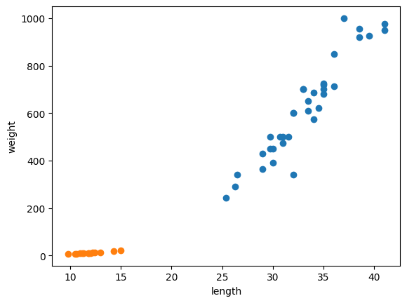
The KNN algorithm predicts the value with the highest frequency by referencing neighboring data points.

Superficially, the closest points seem to be those related to weight. However, weight increases in units of 200, while length is represented in units of 10 on the graph. Therefore, while they might appear closer on the graph, in actual calculation, they are much closer to tomatoes.

Scale Issues #

This problem arises because the x and y data sets in the training set have different scales.

Therefore, we need to preprocess this data by converting it to standard scores.

Standardization: Transforms data to have a mean of 0 and a variance of 1.
Normalization: Scales vectors to have a magnitude of 1.
Robust Scaling: Utilizes the median and IQR (Interquartile Range).

Now, let's look at the code for preprocessing data using standardization.

1. Variance #

\sigma^2 = \frac{1}{n} \sum_{i=1}^{n} (x_i - \mu)^2

2. Sample Variance #

s^2 = \frac{1}{n-1} \sum_{i=1}^{n} (x_i - \bar{x})^2

3. Standard Deviation #

\sigma = \sqrt{\sigma^2} = \sqrt{\frac{1}{n} \sum_{i=1}^{n} (x_i - \mu)^2}

By subtracting the mean from the data, squaring the result, and then taking the average, you can calculate the variance. The square root of the variance is the standard deviation.

import numpy as np
import matplotlib.pyplot as plt
from sklearn.preprocessing import StandardScaler
from sklearn.linear_model import LogisticRegression
from sklearn.model_selection import train_test_split
from sklearn.metrics import accuracy_score

# 1. 가상 데이터 생성 (무게, 색상 점수)
# 사과: 무게 가볍고 색 점수 낮음
# 토마토: 무게 조금 더 무겁고 색 점수 높음
np.random.seed(42)
apples = np.random.normal(loc=[120, 3], scale=[10, 1], size=(50, 2))  # (무게 120g, 색 점수 3)
tomatoes = np.random.normal(loc=[150, 7], scale=[10, 1], size=(50, 2))  # (무게 150g, 색 점수 7)

X = np.vstack([apples, tomatoes])
y = np.array([0]*50 + [1]*50)  # 0=사과, 1=토마토

# 2. 훈련/테스트 분리
X_train, X_test, y_train, y_test = train_test_split(X, y, test_size=0.2, random_state=42)

# 3. 스케일링
scaler = StandardScaler()
X_train_scaled = scaler.fit_transform(X_train)
X_test_scaled = scaler.transform(X_test)

# 4. 모델 학습
model = LogisticRegression()
model.fit(X_train_scaled, y_train)

# 5. 예측 및 평가
y_pred = model.predict(X_test_scaled)
print("테스트 정확도:", accuracy_score(y_test, y_pred))

# 6. 시각화
plt.figure(figsize=(8,6))

# 원본 데이터 산점도
plt.scatter(X[y==0, 0], X[y==0, 1], color="red", label="사과")
plt.scatter(X[y==1, 0], X[y==1, 1], color="green", label="토마토")

# 결정 경계
xx, yy = np.meshgrid(
    np.linspace(X[:,0].min()-5, X[:,0].max()+5, 200),
    np.linspace(X[:,1].min()-1, X[:,1].max()+1, 200)
)
grid = np.c_[xx.ravel(), yy.ravel()]
grid_scaled = scaler.transform(grid)
Z = model.predict(grid_scaled).reshape(xx.shape)
plt.contourf(xx, yy, Z, alpha=0.2, cmap=plt.cm.RdYlGn)

plt.xlabel("무게(g)")
plt.ylabel("색 점수")
plt.legend()
plt.title("사과 vs 토마토 분류 (Logistic Regression + StandardScaler)")
plt.show()

TODO: Need to look up a few scikit-learn functions.